Image classification using CNNs

2021-05-17

CNN , image classification

In this first project, I want to explore image classification using Convolutional Neural Networks (CNNs). CNNs are a type of neural network that has been proven to work well with image data since they account for the fact that adjacent pixels share similar properties and allows the image to be downsampled without losing valuable information. This approach was first presented by Yann LeCun et al (1998) using LeNet-5 to classify handwritten digits.

Overview

The CNN architecture is made up of different layers stacked together. The 3 main components are:

Input layer: this is made up of the input data. Since I am using the CIFAR-10 data, the input data has dimensions 32x32x3 (32 height, 32 width, 3 depth aka. color channels).
Hidden layers: these are the layers in the network made up of the convolutional layers, the activations and the pooling layers. I will explore these different types below and give some examples of different ways of stacking these in the network to achieve better accuracy.
Output layer: a fully connected layer where each neuron is connected to all neurons in the previous layer. For the CIFAR-10 data there are 10 neurons in the output layer, each one corresponding to an output label.

Convolutional layers

Convolutional layers are the core component of CNNs. The output of the conv layer is called the feature map. Each unit in a feature map corresponds to an area in the input data called the receptive field, where the dimension of the receptive field corresponds to the filter size. This filter has dimension FxFxK where F is the length and width and K is the number of channels. Common values of F are 3 or 5.

This filter convolves horizontally and vertically over the input to generate the feature map, computing the dot product between the filter weights and the input values. Each channel within the feature map uses the same set of weights. Doing so helps to dramatically reduce the number of parameters used in the model. The different channels uses a different set of weight, which enables the feature map to extract different features from the image.

Multiple conv layers can be stacked over one another. Here I stack 3 conv layers:

input_shape = (32, 32, 3)
filter_size = (3, 3)

# Build model: add filter and channels
model = Sequential([
    Conv2D(32, filter_size, input_shape=input_shape),
    Conv2D(64, filter_size),
    Conv2D(64, filter_size),

Activation function

The output of the convolutional layer is fed into the activation function. The activation function allows the model to learn nonlinear functions, allowing the network to represent more complex relationships in the data.

In the hidden layer, the 3 most commonly used activation functions are ReLU, Sigmoid and Hyperbolic Tangent. ReLU is preferred over the other activation functions because it is not as prone to the vanishing gradients problem as the others. ReLU is given by the function max(0, x) i.e. where x is returned unless x is less than 0, then 0 is returned. Usually in the hidden layer, the same activation function is used throughout.

Here I use ReLU in each of my conv layers:

input_shape = (32, 32, 3)
filter_size = (3, 3)

# Build model: add ReLU activiations
model = Sequential([
    Conv2D(32, filter_size, input_shape=input_shape, activation='relu'),
    Conv2D(64, filter_size, activation='relu'),
    Conv2D(64, filter_size, activation='relu'),

Activations are also used in the output layer and the activation function used is dependent upon the type of problem being solved. If the problem is a binary classification, then a sigmoid activation should be used whereas if the problem is a multiclass classification, the a softmax activation should be used.

Since the CIFAR-10 data has 10 class labels, I use a softmax activation.

Dense(num_classes, activation='softmax'),

Pooling layers

The pooling layer downsamples the data by reducing the dimension of the feature map by combining small areas together, therefore making it less sensitive to distortions in the data. This means that detecting a specific feature is not dependent upon the precise location of the feature. The 2 commonly used types are:

max pooling: takes the maximum value of the local area or
average pooling: takes the average value of the local area.

I use max pooling, which has been shown to perform better than average pooling, with a 2x2 filter size. Using this filter size with a stride of 2 reduces the dimension of the feature map by a half.

input_shape = (32, 32, 3)
num_classes = 10
filter_size = (3, 3)
pool_size = (2, 2)

# Build model: add max pooling
model = Sequential([
    Conv2D(32, filter_size, input_shape=input_shape, activation='relu'),
    MaxPooling2D(pool_size=pool_size),
    Conv2D(64, filter_size, activation='relu'),
    MaxPooling2D(pool_size=pool_size),
    Conv2D(64, filter_size, activation='relu'),
    MaxPooling2D(pool_size=pool_size),
    Flatten(),
    Dense(num_classes, activation='softmax'),
])

Initial implementation

Training the CNN outlined in the previous section for 10 epochs on the 50k CIFAR-10 training dataset, I achieved an accuracy of 62.3% on the 10k test set. The full code can be found in the section Initial Network: 3 x (CONV -> POOLING) layers in my notebook here.

Next I wanted to explore ways in which I can improve the accuracy of the model.

Channels in the conv layers

The input images have 3 color channels. In each of the subsequent conv layers, the feature map size F decreases. Therefore by increasing the number of channels with each conv layer allows the network to learn a different feature from the data.

Here I increased the channels in the 3rd conv layer from 64 to 128:

input_shape = (32, 32, 3)
num_classes = 10
filter_size = (3, 3)
pool_size = (2, 2)

# Build model: increase channels
model = Sequential([
    Conv2D(32, filter_size, input_shape=input_shape, activation='relu'),
    MaxPooling2D(pool_size=pool_size),
    Conv2D(64, filter_size, activation='relu'),
    MaxPooling2D(pool_size=pool_size),
    Conv2D(128, filter_size, activation='relu'),
    MaxPooling2D(pool_size=pool_size),
    Flatten(),
    Dense(num_classes, activation='softmax'),
])

This resulted in an improvement in the test accuracy from 62.3% to 66.6%.

Batch norm

Batch Normalization standardizes the data to have a mean of zero and standard deviation of one and makes the network quicker to train. Imbalanced data can cause instability in the network, causing imbalanced gradients, which results in the exploding gradient problem. Batch norm can be added to standardize the input data or data in the hidden layers. This normalization happens for each batch separately.

I added batch norm between the initial convolutional layer and max pooling layer to normalize the output from the activation function.

input_shape = (32, 32, 3)
num_classes = 10
filter_size = (3, 3)
pool_size = (2, 2)

# Build model: add batch norm
model = Sequential([
    Conv2D(32, filter_size, input_shape=input_shape, activation='relu'),
    BatchNormalization(),
    MaxPooling2D(pool_size=pool_size),
    Conv2D(64, filter_size, activation='relu'),
    MaxPooling2D(pool_size=pool_size),
    Conv2D(64, filter_size, activation='relu'),
    MaxPooling2D(pool_size=pool_size),
    Flatten(),
    Dense(num_classes, activation='softmax'),
])

This resulted in an improvement in the test accuracy from 62.3% in the initial implementation, to 69.3%.

Fully-connected layer

The role of the convolutional layers is to learn individual features from the data. Adding another fully-connected layer before the final output layer is a way of allowing the network to learn non-linear combinations of features from the convolutional layers.

I added batch norm between the initial convolutional layer and max pooling layer to normalize the output from the activation function.

input_shape = (32, 32, 3)
num_classes = 10
filter_size = (3, 3)
pool_size = (2, 2)

# Build model: add fully-connected layer
model = Sequential([
    Conv2D(32, filter_size, input_shape=input_shape, activation='relu'),
    BatchNormalization(),
    MaxPooling2D(pool_size=pool_size),
    Conv2D(64, filter_size, activation='relu'),
    MaxPooling2D(pool_size=pool_size),
    Conv2D(64, filter_size, activation='relu'),
    MaxPooling2D(pool_size=pool_size),
    Flatten(),
    Dense(64, activation='relu'),
    Dense(num_classes, activation='softmax'),
])

This resulted in an improvement in the test accuracy from 62.3% in the initial implementation, to 65.7%.

Dropout

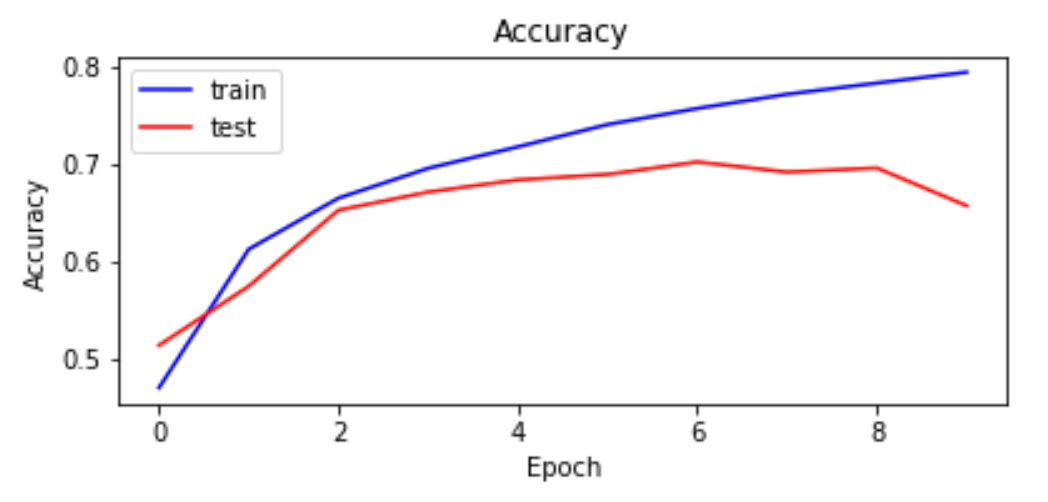
After adding the fully-connected layer, there seems to be some overfitting since the accuracy on the training set improves with each epoch but the accuracy on the test set deteriorates beyond epoch 8. To mitigate this, I added a dropout after the fully connected layer. Dropout helps to avoid overfitting in the network by randomly ignoring some of the layer outputs. As a result the network tries to learn sparse representation from the layer, which helps to prevent overfitting.

input_shape = (32, 32, 3)
num_classes = 10
filter_size = (3, 3)
pool_size = (2, 2)

# Build model: add dropout
model = Sequential([
    Conv2D(32, filter_size, input_shape=input_shape, activation='relu'),
    BatchNormalization(),
    MaxPooling2D(pool_size=pool_size),
    Conv2D(64, filter_size, activation='relu'),
    MaxPooling2D(pool_size=pool_size),
    Conv2D(64, filter_size, activation='relu'),
    MaxPooling2D(pool_size=pool_size),
    Flatten(),
    Dense(64, activation='relu'),
    Dropout(0.5),
    Dense(num_classes, activation='softmax'),
])

Final Model

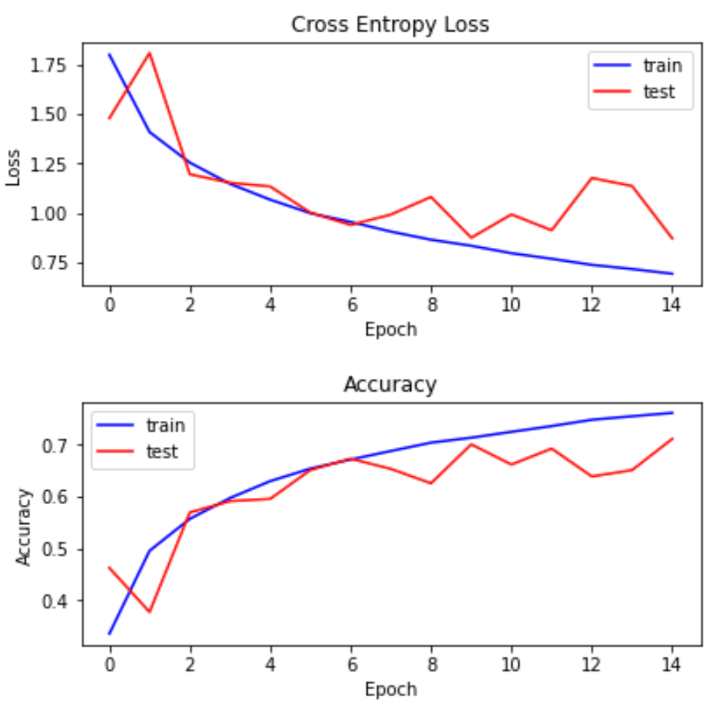
Training the CNN outlined in the previous section for 15 epochs, I achieved an accuracy of 71.1% on the test set. The full code can be found in the section Add dropout to fully connected layer in my notebook here.